Dynamic Rope

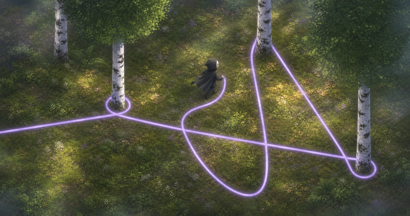
Synopsis

Wrapping rope sounds simple: run a particle simulation, push each particle out of any solid it penetrates, and stroke the chain. The simulation is the easy part. The trouble is that a particle rope resolves every contact through competing forces. A push-out ejects a penetrating particle to the surface, and the distance link to its neighbour hauls it back, often straight back inside. Neither force carries any memory that a contact was already settled, so they never agree and the rope never comes to rest. On a frame where it hasn't, the rope can slip onto the wrong side of an obstacle, and nothing in the simulation knows it was ever meant to be anywhere else. The naive rope is all prevention and no correction.

The fix is to stop asking the particle rope to own topology. A taut-path solver owns side, length, and release; the slack rope only adds shape.

Requirements:

• Wrap, don't clip. Go around the obstacle, on the correct side, with no frame where the rope crosses solid geometry.
• Always know the leash length. The rope pays from a finite spool, so you need the exact deployed length every frame, to stop the player at the limit, or to flash a "taut" warning.
• Release without teleporting. When the player doubles back the rope must unwind, never jump across the obstacle to the wrong side.
• Stay cheap. Every frame, every rope, never the bottleneck.

Terms:

Topology

Which obstacles the rope goes around, and on which side: not the exact shape, just the routing.

Taut path

The shortest route from the spool end to the player end for a fixed topology: straight chords between wraps, and a tangent→arc→tangent around each obstacle. Its length is the taut length: the least rope that reaches the player with those wraps in place.

Winding

How many times, and which way, the rope has gone around an obstacle: a signed turn count carried frame to frame. It is the source of truth for which side the rope is on and how many laps it has made.

Wrap / release

A wrap is the rope catching on an obstacle as the player sweeps around it (winding grows); release is it letting go as the player reverses (winding unwinds and the straight path is clear again).

SDF

Signed distance field: a function giving the distance from any pixel to a shape, used to draw a crisp anti-aliased stroke without tessellating a mesh.

Roadmap: Solve → Simulate → Stroke. First, the failure that motivates the split.

Failure 1: jitter that never settles

Each iteration: push-out shoves a penetrating particle to the rim. The distance-link to its neighbour immediately pulls it back, often back inside. The two constraints fight without memory of "this contact is resolved." The rope buzzes against the obstacle forever.

The chart plots the largest correction any particle takes on each solver iteration, for a ring resting against a disc. A solver settling into a stable state drives this toward zero, with less to fix on every pass. This one does not: push-out moves a particle to the rim, the link pulls it back, and the next pass has the same amount to undo. The correction holds roughly flat across the run rather than decaying, and that is the buzz you see in the rope. (The plot prints the ratio of the last quarter's average correction to the first quarter's; near 1 means no decay.)

Failure 2: a snapshot cannot tell which side

A pure particle sim must ask "is this particle left or right of the obstacle?" from its current position alone. The answer is a sign test, but sign tests are stateless. A single timestep that is too coarse lets a particle tunnel through the disc: it was above before the step, below after, and the sim never saw it cross.

One coarse step (2.5× the obstacle radius) flips the side-readout from +1 (above) to −1 (below), while the true topology never changed. Shrinking a fixed timestep only moves the failure threshold; robust handling needs swept/continuous collision or a persistent winding count.

Failure 3: push-out cannot count laps

A penetration test only knows "this particle is inside right now." It cannot tell how many times the rope has gone around the obstacle. When the rope is double-wrapped (two full loops, with every particle outside the disc), push-out reads zero penetrations, so it finds nothing to correct.

Without a lap count, release can't know how far the player must retrace before the rope should let go. Let go too early and the rope snaps straight through the solid in one frame, teleporting to the wrong side.

A 48-particle double wrap gives push-out lap count 0; integrated winding gives ≈ 2.00 turns.

Defining the winding number

Stand at the center of an obstacle and watch the rope pass by. Each time the rope makes a full counter-clockwise circuit around you, the winding number increases by 1. Each clockwise circuit decreases it by 1. Partial arcs contribute proportionally. Formally, the winding is the total signed angle swept by consecutive vertex-to-vertex rays (a signed angle in radians) which the code divides by 2π to convert to turns:

windingTurns = windingAbout(pts, center) / (2*PI)
  where windingAbout returns signed radians:
  Σ atan2(cross(vᵢ, vᵢ₊₁), dot(vᵢ, vᵢ₊₁))
  where vᵢ = pts[i] − center

In the half-turn pose (≈ 0.5 turns), the gold rays fan out from the obstacle center to each rope vertex; as you move along the rope the rays rotate and the running tally climbs.

Full-turn example

The full-turn pose (≈ 1.0 turns) shows the player routed all the way around the obstacle and back. The winding readout doubles: a visibly distinct number that the solver can act on to distinguish a half turn from a full one.

Why an open path has no side, only a closed loop does

"Which side of the obstacle is the rope on?" sounds answerable from the rope alone, but it is not. A single open path from spool to player has no side: slide any segment left or right and the rope is still the same path from spool to player. There is no fact of the matter encoded in the strand itself.

A side label isn't absolute for an open rope. To compare two routes, close the rope against a chosen reference path and measure that loop's winding. The rope from spool to player (going forward) and the straight chord (the direct straight line) from player back to spool form such a loop. Its winding number around the obstacle center is the exact, unambiguous answer: 0 = same side as the chord, ±1 = one full lap apart, ±2 = two laps, etc.

Why naive per-bead chords give false positives

Tempting shortcut: draw a chord from each rope vertex to a reference line, then flag any chord crossing the disc. The problem: whether that arbitrary line clips the disc says nothing reliable about side.

The chord-falsepos pose shows this exactly. The rope (purple) arcs over the top of the obstacle to reach the player. The dashed grey line is the naive direct chord from spool to player. The closed loop formed by the rope going forward over the top and the direct chord going back underneath winds exactly 0 turns around the obstacle: the rope is topologically fine. Yet the per-bead chords (connecting each rope vertex to its corresponding point on the direct chord) cross the disc and light up red. A naive corrector acting on those red flags would needlessly drag the rope through the obstacle, producing the exact jitter the solver is designed to prevent.

With a valid obstacle-avoiding reference path, the closed-loop winding avoids these per-bead-chord false positives because it uses only the rope and the reference themselves: no arbitrary chord is introduced.

update(playerPos, obstacles)

A fast move could tunnel past a circle between frames, so the update first substeps the endpoint's motion into pieces no larger than half the smallest scene feature (here, half the smallest obstacle radius), and keeps the endpoint in free space (projected out of any disc it lands in). Each substep:

1. Accumulate the winding. For every active wrap, add this substep's change in signed contact span: how its two rope legs rotated relative to each other (Step 2). Done before any topology edit, so the delta reflects real player motion.
2. Converge the topology. Insert a wrap wherever a leg now first crosses an un-wrapped obstacle; release any wrap that has unwound and whose straight chord is clear. Repeat until nothing changes; a single move can catch one obstacle and free another.
3. Rebase. After any insert or release, reset each wrap's stored leg angles to the current geometry without changing its accumulated span, so editing the topology never registers as a phantom turn of winding.

Step 1: the two tangent lines

From the previous node (spool or prior wrap exit) to the obstacle disc, there are exactly two straight lines that graze the disc without crossing it: the external tangents (each tangent line touches the circle at exactly one point without cutting through it). The angle from the point to each tangent contact is:

offset = acos(r / |d|)

where r is the disc radius and |d| is the distance from the point to the disc center. The two tangent contacts sit at angles atan2(d) ± offset on the circle. The same construction runs from the next node (player or next wrap entry) to get two tangent contacts on the exit side.

Obstacles are drawn as circles throughout because the tangent points and arc length come out as clean formulas. Nothing downstream depends on the shape: the same machinery wraps any convex hull (the tangent contact becomes a support vertex) or a boundary loop, see §Synthesis. The circle is the special case that keeps the math readable, not a restriction.

Step 2: which side, and the entry/exit tangents

When a leg first crosses an obstacle, the new wrap takes the side the obstacle was on as the player crossed it: the sign of cross(chord, center − start) using the player's position before the substep, so a fast step can't land the post-move chord on the wrong side and pick backwards. Side in hand, the entry and exit contacts are the two deterministic tangents for that side: the entry is the side's tangent toward the previous node, the exit the opposite-side tangent toward the next. No per-frame search over candidates, so the route can't flicker between equally-scored options, and the leg meets the arc at exactly the tangent point (no gap).

Tracking the winding: the accumulated signed span

Each wrap stores one number: its signed contact span, the running total of how far the rope has wound around that obstacle (CCW +, CW −). Each substep it grows by the relative rotation of the two legs:

span += Δ(exit-leg angle) − Δ(entry-leg angle)

One leg moving (the player) winds the wrap; both rotating together (a rigid pan) does not. This span is the winding memory: it can grow past a full revolution (genuine multi-lap), and a wrap is released only once it has returned toward zero and the straight chord between its neighbours is clear and the release wouldn't flip the rope to the obstacle's far side. Because the span is accumulated rather than re-measured each frame, the solver stays on the consistent side as the player moves instead of snapping to whatever route looks shortest this instant.

(The §Winding point still holds: the span tracks multi-lap winding directly, and the arc renderer draws it as a coil, snapped to the nearest whole lap, so exact through about one turn.)

Step 3: the arc

The winning entry and exit contact angles define an arc on the disc. The rope polyline is assembled as:

[spool, entry, …arc samples…, exit, player]

The arc samples are taken at the same (angle, radius, center) parametrization as the entry/exit points, so the end of the incoming leg and the start of the arc are the same point by construction, no gap.

Taut length: why the arc length matters

The total length of this polyline (leg₁ + arc + leg₂) is the taut length: the minimum rope needed to reach the player with this particular wrap. It is not the straight-line distance from spool to player; a wrap always adds the arc to the bill. Arc length is computed analytically as radius · |span| (not by summing chord samples) so the arc length is analytic, not estimated from samples.

A real tether pays from a finite spool. The solver compares taut length against rope paid out to know:

• Whether the player can move further (taut length < deployed → slack remains).
• When to stop the player or pull the rope taut (taut length = deployed → leash at limit).
• How much slack the rope carries (slack = deployed − taut, the rope paid out minus the taut path).

The API surface for this is solver.tautLength, a getter on PathSolver that returns the sum of straight-leg lengths plus each wrap's arc length (radius · |span|), exact through about one turn (the multi-lap arc rides the nearest-lap span; see §Winding). Read it after every solver.update() call alongside solver.nodes.

Gate 1, unwound: the winding has retraced to a graze

Each wrap carries a signed winding: how far the rope has turned around the obstacle, accumulated as the player moves (positive one way, negative the other, and growing past a full turn for a multi-lap wrap). This is the quantity the gate watches, not the rendered contact arc. As the player wound, the winding grew; as they reverse, it shrinks back toward zero. The wrap releases once the winding has retraced to a graze: for a counter-clockwise wrap, winding ≤ +RELEASE_ANGLE; for a clockwise wrap, winding ≥ −RELEASE_ANGLE (≈ 8.6°).

The gate is deliberately signed, not |winding|. A |winding| test looks safer, but it would keep holding a wrap that unwound past the graze and began winding the other way, exactly the case that should release and re-form on the new side. The signed winding lets go the moment the original wrap is spent.

The rope is still well wound: the winding is far from the threshold, so gate 1 blocks release.

Gate 2, chord clear: straight path does not hit the obstacle

Even after unwinding, the straight chord from the previous node to the next node might still clip the disc, for example, if the rope approaches the obstacle nearly tangentially. Attempting to release in that case would immediately re-trigger a wrap detect on the very same frame. Gate 2 prevents the bounce: if the chord hits the disc, keep the wrap.

Fully unwound, chord clear: all three gates pass, and the rope collapses to a straight chord.

Gate 3, anti-teleport side check

The failure case:

1. The rope winds over the top of the obstacle. The solver stores the wrap's side, say, left of the chord.
2. The player moves back. The winding shrinks to near zero (gate 1 passes).
3. The player ends up on the far side of the obstacle from the spool, so the chord now wants to cross from left-of-obstacle to right-of-obstacle: the opposite side from where the rope was wound.
4. The chord does not clip the disc boundary (gate 2 passes: the chord is geometrically clear). Gates 1 and 2 are both green.
5. Without gate 3, the solver releases the wrap and draws that chord, snapping the rope across the obstacle to the wrong side in a single frame. The chord never passes through solid, but the rope's whole route jumps from one side of the disc to the other instantly.

Gate 2 (chord-clear) and gate 3 (side match) are distinct. Gate 2 asks: "would the replacement chord physically intersect the disc?" Gate 3 asks: "is the replacement chord on the same side of the obstacle that the rope was wound on?" The dangerous scenario above passes gate 2 (the chord misses the disc) but fails gate 3 because the chord is on the opposite side. Gate 3 compares the chord's cross-product side (the sign of cross(next − prev, center − prev), positive if the obstacle center is to the left of the chord, negative if to the right) against the wrap's stored side and vetoes release when they disagree, which stops the rope from teleporting across the disc in a single frame.

With gate 3 disabled, the released chord (red) passes below the disc. It clears the obstacle, but lands on the wrong side. The faint purple arc is the correctly held wrap.

Beyond circles: hulls and boundary loops

Every demo here draws obstacles as circles because a circle's tangent points and arc length come out as clean formulas. Nothing in the architecture depends on that shape. The same wrap machinery handles a convex hull: the analytic tangent point becomes a support vertex (occasionally a whole edge), and the circular contact arc becomes the chain of hull edges the rope actually touches. The legs are still tangents; the topology (which obstacle, which side, how far wound) is tracked exactly as before.

This is the same construction from §Solve, with the circle swapped for a polygon. The reusable solver in this repo stays circle-only on purpose (analytic and readable); generalising the contact test to support vertices is the one piece a fuller implementation adds.

A boundary loop is the same wrap, inside-out

A boundary loop is the rope routed around the inside of an enclosing region, hugging the rim of a pit or a cleared area instead of the outside of an obstacle. It uses the same winding bookkeeping with the admissible side reversed: an inward corner of the boundary is, locally, just a convex hull vertex seen from the other side. Wrapping outside an obstacle and wrapping inside a loop are the same mechanism.

So circles, convex hulls, and simple boundary loops are a single collision problem; the topology state (which side, how far wound) stays identical.

Verlet integration carries the shape: store each particle's current and previous position rather than an explicit velocity, and extrapolate forward each step:

new_pos = pos + (pos − prev_pos)

It is numerically stable and needs no velocity bookkeeping: velocity falls out of the positional difference. Crucially, the particles remember where the rope has been: that memory is what lets the slack hold the shape it was deployed into, instead of snapping onto the chord.

One-sided distance links

Adjacent particles are joined by one-sided distance links: if two particles are pulled further apart than the rest length, the link pulls them back together; if they drift closer, it does nothing. That asymmetry is what makes a rope and not a rod: the chain can never stretch past its material length, but it is free to bunch up and bow into slack. A few iterations of constraint relaxation per frame keep the links satisfied.

So once the hand retraces, the deployed material is longer than the straight chord to the player: the links can't pull it taut, and the leftover length bows out into the slack curve in the figure.

Redistributing the slack

The one-sided links resist only stretch, so the rope is free to go slack, but they never say where along the curve the surplus should sit, and a chain of one-sided links can pile material unevenly wherever a link happened to give. A redistribution pass can even this out: resample the chain to uniform arc-length along its own curve, sliding particles tangentially so the shape is untouched but the spacing is regular. This in-plane explainer runs without it. Resampling a flat 2D curve to uniform spacing pulls the bowed slack back toward the straight taut path and flattens the loop, and the Bézier stroke evens the spacing at render time anyway, so the demos keep the raw chain. The shape itself is pure memory: the slack holds whatever curve the hand laid it in, bowing into an in-plane loop where the hand moved off the straight line, because nothing pulls an in-class bead back onto the taut path. Material is conserved either way: redistribution only slides particles along the rope, it never adds or removes any.

Keeping the slack rope in the taut path's winding class

The naive rope never solved this: a slack particle sim can drift to the wrong side of an obstacle the taut path wraps. When that happens the two ropes disagree about topology, and the rope you draw is wrong: it cuts through a trunk the taut path went around, or hangs on the wrong side of a wrap.

The naive fix ("snap any bead that's on the wrong side back") is exactly what §Naive showed flickering. A per-bead side test has no memory and no global picture. Ask the global question instead: is the slack rope in the same winding class as the taut path?

loopK: the winding class

Take the total signed turning of each rope about the obstacle's centre: the sum of the angle each segment sweeps, CCW positive, CW negative. The slack rope's turning minus the taut path's, over 2π and rounded, is an integer:

loopK = round( ( winding(slack) − winding(taut) ) / 2π )

loopK = 0 means the two ropes are in the same class: same laps, same side. loopK = ±1 means the slack rope has slipped one full loop off the taut path. That single integer is the entire correctness test.

Lobes and winding defects: where it slipped

loopK says the rope slipped; lobes say where. Find where the slack rope crosses the taut path. Between two consecutive crossings is a lobe: a closed loop of a slack arc and the taut arc back. Each lobe carries its own integer winding defect: the net turns that lobe makes around the obstacle. The beads in a lobe whose defect is nonzero are the ones that slipped; they are pulled back toward their material bookmark on the taut path.

Bookmarks: pulling a bead home along the rope

Which point should a slipped bead be pulled toward? Not the nearest point on the taut path: that can sit on the far side of a trunk, and snapping there teleports the rope across the obstacle. Each bead instead carries a bookmark: its own material coordinate M, its arclength position along the deployed rope (0 at the spool, the full deployed length at the hand). Its bookmark is the taut-path point at arclength U = M · min(1, taut/deployed): when the rope is slack the factor taut/deployed packs the material evenly onto the shorter geodesic; when it's taut the factor is 1 and U = M. Either way the bookmarks tile the taut path in the same order the beads run along the rope, a frame-to-frame correspondence between the slack rope and the geodesic.

Correcting a wound bead is a three-way decision. If the bead sits inside an actionable trunk, it is first evicted straight out along its chord to the rim, so it never tunnels through. Otherwise, if the chord to its bookmark (or an adjacent rope segment) crosses an actionable trunk, it is pulled a bounded step toward its bookmark; and if neither holds, it is left alone. Because the bookmark is the matching material point, a pulled bead returns along the rope's own length: it unwinds the way it wound, rather than cutting across the trunk. The §Synthesis capstone draws these correspondences live: every line ties a slack bead to its bookmark on the taut path, and when a lobe is out of class the lines turn red and reel it back in.

A lobe is acted on only when Actionable(defect, loopK) = defect ≠ 0 AND loopK ≠ 0. Drag the rope under the trunk in the figure: the class flips to loopK = 1, the lobe lights up with defect +1, and the wound beads sprout pull-back arrows toward the geodesic. Drag it back over the top and the class returns to 0, nothing to correct. (This figure isolates the loopK gate and the bookmark pull-back; the full three-way repair, including the eviction of a bead caught inside a trunk, straight out along its chord to the rim, runs in the slack-rope sim, shown live in the §Synthesis capstone.)

Why gate on loopK: tangency flicker

The global loopK ≠ 0 gate prevents tangency flicker. At grazing contact, when the slack rope barely kisses an obstacle, it crosses the taut path several times and splits into several lobes, and a per-lobe test twitches every frame as those crossings appear and vanish. But the rope's global winding class doesn't move: the slack is still the same class as the taut (loopK = 0). Gating on loopK ≠ 0 kills the flicker: if the global class is zero, there is nothing to fix, whatever the lobes say. In the figure the slack grazes the trunk and splits into several lobes, all in the same winding class (loopK = 0), so not one bead is touched.

The conservation check

Lobe defects should sum to loopK. In a clean diagram they do, exactly; it's how you know the lobe split is consistent with the global class. In a real-time sim's noisier geometry it's a diagnostic rather than a hard gate. One more wrinkle: once a correction starts, a lobe's explicit crossings can vanish mid-pull while the rope is still a lap off, so a bookmark-discrepancy fallback keeps drawing those residual beads home until the class actually reads zero.

None of this lives in the textbook tangent-and-arc solver. It is the accumulated scar tissue of making a slack, swinging rope agree with a taut geometric one, frame after frame, without flicker.

Dead end 1: decimate then globally fit

First attempt: run Douglas–Peucker decimation on the particle chain, then fit a global smoothing spline.

This breaks by control-point starvation. Straight legs dominate the arc-length budget. The figures compare a low control count (8) against a high one (64): almost all controls land on the legs, leaving the tight wrap with one or two controls to describe a half-circle whose chord deviates ~300 mm from the true arc. Even at 64 controls the error is still ~65 mm. The improvement is a 4.6× factor that still isn't good enough.

A second problem compounds this: decimation's kept-set is unstable. Tiny perturbations of the rope's particle positions flip which points survive the threshold, causing the fit to jump discontinuously between frames.

Dead end 2: a polynomial spline cannot be a circular arc

The second idea: fit the wrap region with a degree-2 polynomial spline. This is a mathematical limit, not an engineering tradeoff.

A circular arc is a conic section; it cannot be represented exactly by any polynomial of finite degree. A quadratic polynomial matches the arc only at its endpoints and one other point; between those, it deviates and oscillates. The more segments you add to reduce the oscillation, the more control points you need, which reintroduces the starvation problem from dead end 1, now at the segment seams instead of the whole wrap.

The solver already knows the arc parameters exactly

Both dead ends assume the arc must be recovered from the particles. It need not be: the solver already computed every wrap's exact parameters: (center, radius, a0, a1). That information is still in memory, so instead of fitting a curve to noisy beads, we tessellate the known arc directly. That trades an unbounded fitting error for a small, bounded tessellation error (≈0.06%·r at 30° per Bézier, close, not mathematically exact).

Per frame:

1. Decompose the corrected sim polyline into arc spans and free spans.
2. Tessellate arcs from (center, r, a0, a1) into quadratic Béziers. At 30° per segment, error is ≈0.06% of radius.
3. Fit free spans from particle samples with centripetal Catmull-Rom, converted to quadratics.
4. Draw the stroke with a per-fragment SDF over the Bézier set.

The module split

The stroke is built in three steps: decompose the rope into the spans that hug a wrap (arcs) and the spans that don't (free), tessellate each arc to quadratic Béziers, and fit each free span to a smooth Bézier that joins the arc tangentially. Drag the slack handle: as a free leg flexes with in-plane slack, it stays anchored to (and tangent with) the arc at the contact points.

The SDF stroke in action

A single quadratic Bézier rendered as an SDF stroke. Switch to the cpu or heatmap pose (via the URL) to see the Canvas 2D fallback and the distance-field colour ramp: bands of colour varying smoothly outward from the stroke boundary are the verification signal that the field is correct.

Pixel coordinates: a 3D renderer's shaders avoid backend Y-flips by passing a projected v_px varying. This demo works directly in pixel space.

Synthesis

One frame: solve, simulate, stroke.

Frame pipeline

2D vs 3D

The topology problem is planar. The solver works in the ground plane (the two horizontal axes): obstacle containment, winding, tangent choice, wrap insertion, release, boundary loops, and loopK all ignore height. That is the key to keeping it tractable: topology is a 2D question.

The slack rope and renderer are spatial. Each bead carries its two ground-plane coordinates for topology plus a height coordinate for ground contact and camera-facing stroke data. Topology checks project beads back to the ground plane; rendering uses the full position. Crucially, the slack rope's shape is a geometric construct: it is the deployed material (a running max of rope paid out) relaxed against the shortened taut path, so the surplus bows out in-plane (slack = deployed − taut). It is geometry, not a time-based settle or a drag trail, resting on the same conserved-material pillar the winding-class correction follows. (In 3D, gravity additionally settles the already-slack rope into a vertical height; it is not what creates the slack.)

The capstone below is the 2D top-down view: drag the player to wind the trunks, then drag back; the paid-out material (a running max) now exceeds the shortened taut path, so real in-plane slack bows out as a loop. The purple ribbon strokes the slack rope itself; the toggles reveal the taut geodesic it rides, the raw particle chain, and each bead's bookmark (its material point on the taut path). The 3/4 view up top is the same planar solve rendered through an oblique camera (three trunks, the hero arrangement); the projection is the only 3D part.

Game-loop recipe

Frame order:

// path-solver.js: authoritative topology + taut path
solver.update(playerPos, obstacles)

// the taut polyline, [{x,y}], guaranteed outside all obstacles
const taut = solver.nodes

// clamp the player / show a "taut" warning when len >= paidOut
const len = solver.tautLength

// The slack rope's SHAPE is your sim's job. It is MATERIAL, not a drag trail:
//   PAYOUT: pay out rope at the hand. New material inserts just behind the hand; existing beads
//     keep their material coordinate M (never re-indexed). deployed length is a running max.
//   LOCK:   a Verlet/PBD chain conserves that material; a bead LOCKS onto the taut path once its
//     chord error to the geodesic is below eps AND its links are at rest (unlocking on a stretch
//     or a chord jump). Locked beads ARE the taut path; only the slack ones bow.
//   Retracing shortens taut while material is conserved, so the surplus bows out in-plane as slack.
//   (In 3D, gravity only settles the already-slack rope into a vertical height, not the source.)
const sim = updateSlackShape(playerPos, taut, solver.wraps)
// keep it in the taut WINDING CLASS: each bead's bookmark is the taut-path point at U = M*min(1, taut/deployed);
// repair an out-of-class bead by a 3-way rule (evict along its chord if inside an actionable trunk;
// else pull to its bookmark if the chord-to-bookmark OR an adjacent segment crosses one; else skip).
keepInWindingClass(sim, taut, obstacles)

// rope-stroke.js: turn the rope into render-ready quadratic Béziers:
// slackStroke decomposes the SIM rope (primitive-decompose) into arc spans
// (arc-tessellate) + free spans (free-span-fit); tautStroke builds straight
// from the solver wraps when the rope is in its taut class.
const beziers = slackStroke(sim, solver.wraps, { circles: obstacles })

// bezier-sdf.glsl: one SDF pass over the packed Bézier set
drawSdfStroke(beziers)

Function map

Concept to code:

vec2.js

2D vector primitives (add, sub, dot, cross, len, norm, fromAngle, angle).

verlet.js

createRope, step, pinEnd: the Verlet integration loop with one-sided distance constraints (an optional gravity term, off in this in-plane explainer). Owns the shape layer; knows nothing about topology or obstacles.

path-solver.js

PathSolver: the topology engine. Feed it a spool position, call .update(playerPos, obstacles) each frame, read .nodes for the taut polyline and .tautLength for the leash length (exact through ~one turn). Internally: endpoint substeps, deterministic wrap-side insertion from the crossing, accumulated signed contact span, zero-gap tangent/arc parametrisation, topology rebase after edits, and all three release gates (unwound, chord-clear, anti-teleport side check).

slack-topology.js
slack-correction.js

The winding-class correction from §Simulate. slack-topology.js computes loopK, slack↔taut crossings, lobe defects, and the defect≠0 && loopK≠0 gate. slack-correction.js adds the explainer-scale glue: material bookmarks, bookmark-discrepancy fallback, bounded pull-back, and obstacle projection, driving the §Simulate lobe-defect demo. (The capstones run their winding-class correction inside the slack-rope sim itself.)

primitive-decompose.js

decompose(points, wraps): classifies a corrected sim polyline into arc spans (sections near a wrap's contact arc) and free spans (the slack legs between wraps), returning a list of {kind, start, end, arc?} primitives. The bridge between the solver's wrap data and the tessellation / fitting stage. (Each wrap exposes its entry/exit tangent points and signed span; derive the contact-arc start angle as atan2(entry − center) wherever a tessellator wants an angle rather than a point.)

arc-tessellate.js

tessellateArc({center, radius, a0, a1}): converts an exact circular arc into a sequence of quadratic Bézier segments. Each segment's control point is derived from the arc's mid-angle so the approximation error is < 0.1% of the radius regardless of how many segments are used.

free-span-fit.js

fitFreeSpan(points): fits a sequence of particle positions with centripetal Catmull-Rom, converting each span to a quadratic Bézier. Includes an obstacle-avoidance fallback: if any Bézier in the span would push the curve inside a circle, the whole span degrades to straight chords (so a smooth curve never abuts a straight one at a kink).

bezier-sdf.js
bezier-sdf.glsl

CPU and GPU implementations of Inigo Quilez's exact quadratic-Bézier signed distance function. Feed it a fragment position and three control points; get distance to the curve. The GPU path evaluates one Bézier or the nearest of a packed Bézier set, no rope mesh, just SDF anti-aliasing.

rope-stroke.js

tautStroke({anchor, wraps, endpoint}) builds the render-ready quadratic Béziers straight from the solved taut path: each wrap arc consumed with its signed span, so a wrap past a half-turn arcs the correct way and lands on its exit tangent (the multi-lap span is the nearest-lap reconciliation, exact through ~one turn). slackStroke(points, wraps) does the same for a corrected slack rope (decompose → wrap arcs + fitted free spans); the two coincide when the slack rope is in its taut winding class.

camera-ortho.js

makeGroundCamera(...), the 3/4 capstone's only 3D piece: an invertible oblique-orthographic projection of the ground plane (depth foreshortened, obstacles raised into vertical poles). Topology is solved in the ground plane; this just projects the result and unprojects screen drags.

rope-sim.js

The slack-rope sim shared by both capstones as the Simulate stage. A Verlet/PBD chain: one-sided links (resist stretch, allow bunching), material paid out at the hand, lock-to-taut, and the winding-class correction (a bead inside a trunk is evicted along its chord to the rim). Its published points are the slack rope the stroke draws, not a drag trail. Deployed length is a running max, so retracing the player produces real in-plane slack (slack = deployed − taut).

player-paths.js

densify, arcWaypoints, retrace: distance-sampled (frame-rate-independent) recorded player drags. The capstones replay these to seed a pose, and the tests drive them to assert emergent behaviour rather than placed states.

Extending it

Extensions:

• Production-scale correction. The capstone includes the core lobe/defect/loopK correction. A full real-time implementation adds the same engineering around it: broad-phase crossing scans, fixed scratch buffers, contact-pole dispatch, and persistent residual bookmark correction while a wound lobe is collapsing back onto the taut path.
• Non-circular obstacles. Convex hulls and boundary loops (Beyond circles): the same wrap machinery handles a hull (the tangent contact becomes a support vertex) and a free-space boundary (the same wrap, inside-out, around reflex corners). The contact geometry changes; the topology state does not.
• Drawing multiple laps. The winding is already a single accumulated span that grows past a revolution, so multi-lap is tracked for free, and the arc renderer here already draws the extra revolutions (reconciledSpan is lap-aware). What a fuller renderer adds is making that exact past one turn (instead of round-to-nearest-lap) and de-overlapping the stacked coil arcs.